This article is Part 3 in a 3-Part Tensorflow 2.0.
Introduction
In the previous post of this series, we developed a simple feed forward neural network that classified dress types into 10 different categoreis. We were able to achieve accuracy of 86% on test set after training the model for about 10 epochs. In this post, I’ll show how using convolutional neural networks can significantly improve the accuracy of the model when working with images. If you are not familair with how CNNs work then I recommend you read this article from Stanford University CS231n course.
In this post also we’ll use Fashion MNIST dataset. If you need to know more about this dataset, then checkout previous post in this series to get a brief introduction. This post is a walkthrough on the keras example: mnist_cnn. However, the code shown here is not exactly the same as in the Keras example. Specifically, we’ll be using Functional API instead of Sequential to build our model and we’ll also use Fashion MNIST dataset instead of MNIST.
Let’s import required libraries
1
2
3
4
5
6
import numpy as np
from tensorflow import keras
from tensorflow.keras import backend as K
from tensorflow.keras.models import Model, Sequential
from tensorflow.keras.layers import Dense, Dropout, Flatten, Conv2D, MaxPool2D, Input
from tensorflow.keras.datasets import fashion_mnist
Note: I’m using tensorflow 2.0.0-beta1
Data Processing
First thing we need to do is load the data, convert the inputs to float32 type and divide by 255.0 because we want to scale the pixel values so that they lie between 0 and 1. If we look at the shape of input and output, we see that there are 60,000 training images of size 28 x 28 pixels.
1
2
3
4
5
(x_train, y_train), (x_test, y_test) = fashion_mnist.load_data()
x_train = x_train.astype('float32') / 255.0
x_test = x_test.astype('float32') / 255.0

x_train.shape, x_test.shape, y_train.shape, y_test.shape
1
((60000, 28, 28), (10000, 28, 28), (60000,), (10000,))
Now, let’s figure out the input shape and total classes in the dataset
1
2
input_shape = (x_train.shape[1:] + (1,)) # (28, 28, 1)
num_classes = len(np.unique(y_train))
input_shape is a tuple telling the model about the shape of the input it will be getting. Note that instead of (28 x 28) we have the shape as (28 x 28 x 1). This is necessary because 2D CNNs accept 3D input tensors. Since our images are grayscale we need to add a dimension at the end. If our images were colored then their shape would be (28 x 28 x 3), 3 because there are 3 color channels Red, Green and Blue.
Note that tensorflow backend of Keras expects input shape to be in format (height x width x channels), theano backend expects input shape to be (channels x height x width). Other backends like CNTK may have their own format so you should check and adjust accordingly.
Now we need to convert our labels to one-hot encoded form. This is necessary to do this if we use categorical_crossentropy loss when training the model. However if we use sparse_categorical_crossentropy then we can skip this step. If you look at previous post, you’ll see that we are using sparse_categorical_crossentropy loss so the labels were not converted to one-hot encoded form.
1
2
y_train = keras.utils.to_categorical(y_train, num_classes)
y_test = keras.utils.to_categorical(y_test, num_classes)
Model
To define a model, we’ll use Functional API instead of sequential. After input layer, we have two convolutional layers. Both of them have same activation and kernel size but different filters.
1
2
3
4
5
6
7
8
9
10
11
inp = Input(shape=input_shape)
_ = Conv2D(filters=32, kernel_size=(3, 3), activation='relu')(inp)
_ = Conv2D(filters=64, kernel_size=(3, 3), activation='relu')(_)
_ = MaxPool2D(pool_size=(2, 2))(_)
_ = Dropout(0.25)(_)
_ = Flatten()(_)
_ = Dense(units=128, activation='relu')(_)
_ = Dropout(0.2)(_)
_ = Dense(units=num_classes, activation='softmax')(_)
model = Model(inputs=inp, outputs=_)
model.summary()
1
2
3
4
5
6
7
8
9
10
11
12
13
14
15
16
17
18
19
20
21
22
23
Layer (type)                 Output Shape              Param #
=================================================================
input_9 (InputLayer)         [(None, 28, 28, 1)]       0
_________________________________________________________________
conv2d_15 (Conv2D)           (None, 26, 26, 32)        320
_________________________________________________________________
conv2d_16 (Conv2D)           (None, 24, 24, 64)        18496
_________________________________________________________________
max_pooling2d_9 (MaxPooling2 (None, 12, 12, 64)        0
_________________________________________________________________
dropout_18 (Dropout)         (None, 12, 12, 64)        0
_________________________________________________________________
flatten_9 (Flatten)          (None, 9216)              0
_________________________________________________________________
dense_18 (Dense)             (None, 128)               1179776
_________________________________________________________________
dropout_19 (Dropout)         (None, 128)               0
_________________________________________________________________
dense_19 (Dense)             (None, 10)                1290
=================================================================
Total params: 1,199,882
Trainable params: 1,199,882
Non-trainable params: 0
Let’s walkthrough the layers. Pay attention to the model summary specially the Output Shape. The first is the input layers which takes in a input of shape (28, 28, 1) and produces an output of shape (28, 28, 1). Note that the None in the table above means that Keras does not know about it yet it can be any number. In almost all the cases if you see a None in first entry of output shape then its value will be the batch size. For most purpose you can ignore this.
Moving to second layer- the Conv layer. The table shows that the output of this layer is (26, 26, 32). The input to this layer is output from previous layer. So it is taking a (28, 28, 1) tensor and producing (26, 26, 32) tensor. The width and height of the tensor decreases due to a property of conv layer called padding. By default it is set to valid. If it is valid then the output dimension will decrease based on the kernel size. Try changing the kernel size and see how the dimension decreases as you increase the kernel size. However, if padding is set to same then the dimension will not decrease no matter what the kernel size is.
Now what about 32? This is because of the number of filters we specified. Each filter will produce a tensor which are stacked together so in this case 32 filters were applied to the input and each of them produce a tensor of size (26, 26) and when we stack them along the 3rd axis, we get the output of shape (26, 26,32).
Similarly for second conv layer, we see the output dimension has decreased but because there are 64 filters, the shape is (24, 24, 64).
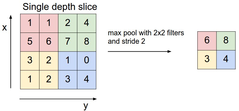
MaxPooling is another operation typically used after convolutional layer to reduce the shape. Figure below shows how it works (taken from here).
Dropout layers are used to randomly drop some activations of the network while training so that the network does not overfit. Dropout layers are only executed during the training process and not during inference. Keras automatically takes care of this. We can specify what percentage of activations to discard as its parameter. I’ve seen people typically use the value between .2 to .3.
Until dropout layer, our tensor is 3D. But for a fully connected layer, we need 1D input. So we use Flatten layer to flatten the output and feed it to the Dense layer.
Training
To train, we should compile the model first. categorical_crossentropy is the loss function to use if we want to do multi-class classification. For optimizer, I’ve chosen Adam but you can change it and see how quick the model converges.
When calling the fit function, we add 1 dimension at the end so that our input shape becomes (60000, 28, 28, 1) instead of (60000, 28, 28).
1
2
3
model.compile(loss=keras.losses.categorical_crossentropy,
              optimizer=keras.optimizers.Adam(), metrics=['accuracy'])
history = model.fit(np.expand_dims(x_train, -1), y_train, batch_size=128, epochs=12, validation_split=0.3)
1
2
3
4
5
6
7
8
9
10
Train on 42000 samples, validate on 18000 samples
Epoch 1/12
42000/42000 [==============================] - 24s 581us/sample - loss: 0.5063 - accuracy: 0.8218 - val_loss: 0.3416 - val_accuracy: 0.8768
Epoch 2/12
42000/42000 [==============================] - 24s 574us/sample - loss: 0.3207 - accuracy: 0.8856 - val_loss: 0.2887 - val_accuracy: 0.8933
...
Epoch 11/12
42000/42000 [==============================] - 24s 580us/sample - loss: 0.1078 - accuracy: 0.9603 - val_loss: 0.2384 - val_accuracy: 0.9238
Epoch 12/12
42000/42000 [==============================] - 24s 580us/sample - loss: 0.0954 - accuracy: 0.9642 - val_loss: 0.2450 - val_accuracy: 0.9239
In the validation set we got accuracy of 92%. This model clearly performs much better than the fully connected one trained in the previous post.
Evaluation
Now let’s evaluate the model on test set
1
2
loss, accuracy = model.evaluate(np.expand_dims(x_test, -1), y_test, verbose=0)
print(loss, accuracy)
1
0.2691077432125807 0.9166
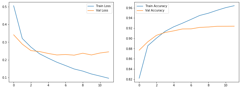
This model achieved 91% on test set which is much better than 87% from the model in previous post. We can also plot the accuracy and loss history while the model was trained.
1
2
3
4
5
6
7
8
9
10
import matplotlib.pyplot as plt
%matplotlib inline

fig, (ax1, ax2) = plt.subplots(nrows=1, ncols=2, figsize=(14, 5))
ax1.plot(history.history['loss'], label='Train Loss')
ax1.plot(history.history['val_loss'], label='Val Loss')
ax1.legend()
ax2.plot(history.history['accuracy'], label='Train Accuracy')
ax2.plot(history.history['val_accuracy'], label='Val Accuracy')
ax2.legend()
Conclusion
To summarize, CNNs perform much better than feed forward networks when working with image data. The most important parameters of CNN layer are filters, kernel_size, padding and activation. There are numerous other parameters that you can tweak. Refer to Keras documentation for more information.
This article is Part 3 in a 3-Part Tensorflow 2.0.


Comments